Discrete probability distribution#
A binomial distribution is actually a special case of a discrete probability distribution since the probability is constant across all the events. When the probability varies across repetitions, the mean (the expected value) is determined by considering all possible values of the random variable, denoted as \(x_i\). Each value is multiplied by its respective probability, \(p_i\), and the products are then summed together.
\(\text{mean} = \mu = \sum_i^{}p_ix_i\)
\(\text{variance} = \sigma^2 = \sum_i^{}p_i(x_i-\mu)^2\)
If each of the individual probabilities, \(p_i\), are plotted, the discrete probability distribution is called a discrete probability density function (or a probability mass function, PMF). A discrete random variable is one that can take on a countable number of distinct values. For each possible value of the random variable, the PMF gives the probability of observing that value.
Key properties of a discrete probability density function include:
For all possible values of \(x_i\), the probability is non-negative, i.e \(p_i \geq 0\).
The sum of the probabilities for all possible values of \(x_i\) equals 1: \(\sum_{i} p_i = 1\).
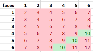
Example. Two six-sided dices are thrown. What is the probability that the sum of the dices is 10?

Fig. 28 All the combinations for the sum of two dices, where green cells represent the favourable events.#
By classical probability, we can compute that
\(P(\text{the sum of two dices is 10})=\frac{3}{36}=\frac{1}{12}\)
EXERCISE 1. Mean and variance for the sum of two dices
Compute the mean and variance for the sum of the faces, when two six-sided dices are thrown.
Answers: mean = 7
variance = 5.8
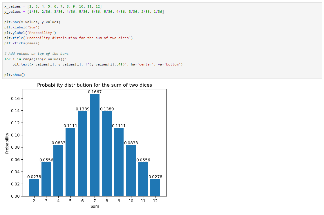
If we draw a distribution of all the possible sums, we have to count the probabilites separately. A Python code could look like this:

Fig. 29 Sum of two dices in a discrete distribution.#
So if the question would be, what is the probability that the sum of the two dices is at most 5, we would have add the probabilities of events ‘the sum is 2’, ‘the sum is 3’, ‘the sum is 4’ and ‘the sum is 5’. That’s when the cumulative distribution funtion comes handy.
Cumulative distribution funtion, CDF#
The cumulative distribution function (CDF) describes the probability that a random variable takes on a value less than or equal to a given value. For discrete random variables, the CDF gives the cumulative probabilities for each possible value.
If we denote the cumulative distribution function by \(F(x_i)\) of a random variable \(x_i\), the notation would be
\(F(x_i) = P(X \leq x_i) = \sum_{i} p_i\)
The value of the CDF at the highest possible variable value is 1, since every value is at most equal to the highest variable value.
The cumulative distribution function satisfies the following properties:
\(0 \leq F(x) \leq 1\) for all \(x_i\)
\(F(x)\) is non-decreasing: \(F(x_1) \leq F(x_2)\) if \(x_1 \leq x_2\)
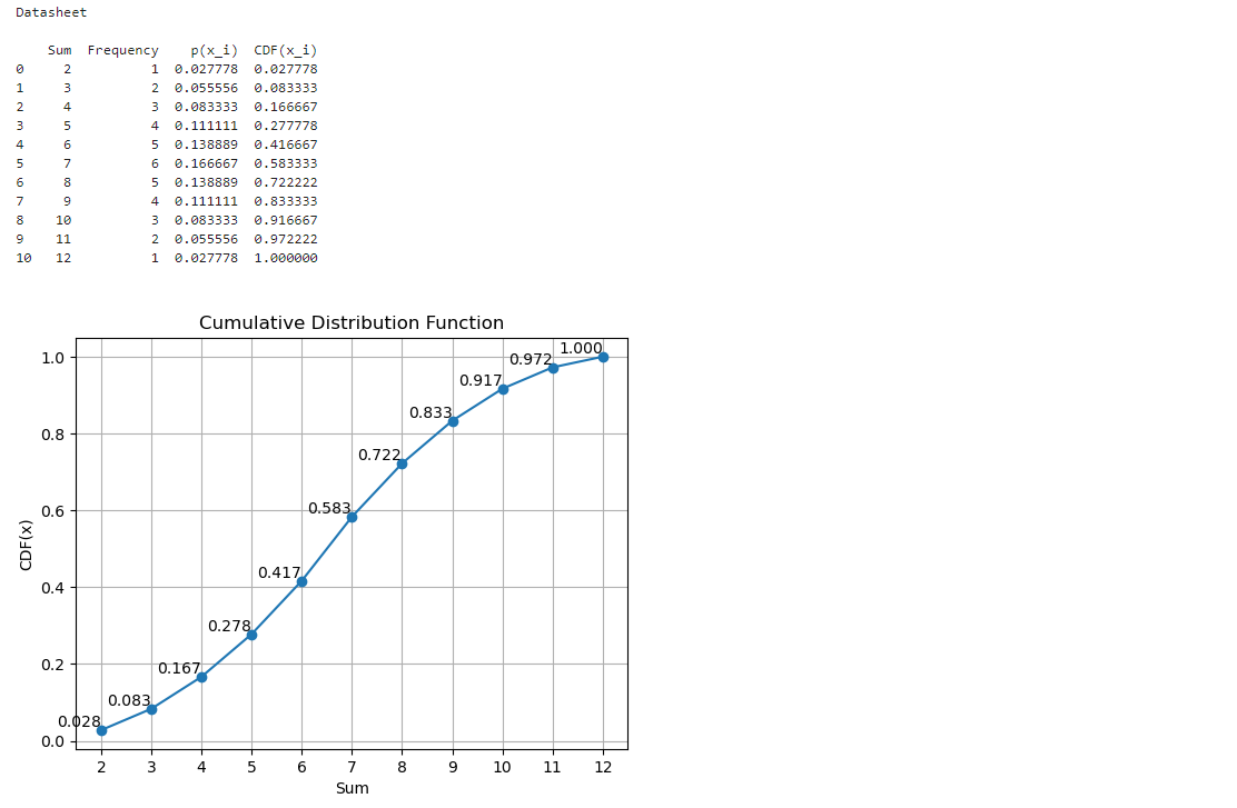
So what is the probability that the sum of the two dices is at most 5? From the CDF we can see that
\(F(5) = P(X \leq 5) = \sum_{5} p_5 = 0.416...\)
In Python, the CDF can computed using the command cumsum from NumPy.

Fig. 30 Sum of two dices in a cumulative distribution function.#
Although the cumulative function describes the probability that the variable value is at most something, it can also be used to calculate that the variable value is at least something. In this case, the complement principle must be used: if the number is greater than 10, then it is not less than or equal to 10.
